• Home
• Programming
• Computer Science
• Twisting Puzzles
• Arduino
• BBC micro:bit
• Raspberry Pi Pico

Computer Science

• Computer Science Home

Data Representation

• Binary Numbers
• Hexadecimal Numbers
• Character Coding Schemes
• Error Detection & Correction
• Bitmapped & Vector Graphics
• Image Compression Techniques
• Sound
• Real Numbers
• Logic Gates - Truth Tables
• Logic Gates - Diagrams
• Boolean Algebra

Program Design

• Principles Of Computation
• Problem Solving
• Hierarchy Charts
• Stepwise Refinement
• Finite State Machines
• State Transition Tables
• Decision Tables
• Algorithm Design
• Structured English
• Pseudocode
• Program Flowcharts
• Dry-Running
• Programming
• Structure Charts
• Structured Programming
• Testing
• Finite State Machines
• Turing Machines
• Types Of Problem
• The Systems Life Cycle

Hardware & Software

• Computer Architecture
• The Stored Program Concept
• Structure Of The Processor
• Machine Code Operations
• The Fetch-Execute Cycle
• Operating Systems
• Input Devices
• Output Devices
• Storage Devices
• Classification Of Software

Networks

• The Internet
• Domain Names & IP
• TCP/IP Protocol
• Web Design
• Communication Methods
• Networks
• Networks 2
• Server-Side Scripting
• Internet & Computer Security

Databases

• Entity Relationship Modelling
• Database Design
• Structured Query Language

Data Structures

• Stacks
• Queues
• Linear Lists
• Linked Lists
• Graphs
• Trees

Algorithms

• Recursion
• Binary Search
• Insertion Sort
• Hashing
• Simulations
• Comparing Algorithms

Other

• Computers & The Law
• Abstraction
• Regular Expressions
• Backus-Naur Form
• Reverse Polish Notation
• Programming Paradigms
• Object Oriented Programming

 

Computer Science
Graphs

A graph consists of a set of vertices and edges. Each edge may have a label, known as its weight or cost.

The London Underground map is probably the most familiar graph diagram that you have seen. If you were to compare the map with the physical locations of the stations, you will see that some liberties have been taken with the geography of the city. The diagram restricts itself to the information that is useful to its users - the connections. On the diagram you can see which stations are connected and work out a route. The distances don't matter so scale is not important in this diagram.

If we consider the transport links between towns in the local area, we might come up with a graph something like the following,

• A - Bishop's Stortford
• B - Braintree
• C - Colchester
• D - Harlow
• E - Chelmsford

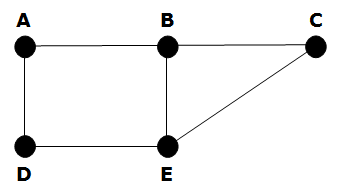
This type of graph is known as an undirected graph. There is no directional information. Notice that there is also no sense of scale and the towns are not in their exact position. This graph merely shows the connections between the vertices. For example, following major roads only, you pass through Braintree on your way to Colchester from Bishop's Stortford.

In this graph, A & B are neighbours because there is a connection between them. A & D are also neighbours. Vertex A is said to have a degree of 2 - it has two neighbours.

The WWW, LANs & WANs, traffic flow, transport links, circuits, chemical compounds, social networks are all examples of real-world situations that lend themselves to being modelled with a graph.

Weighted Graphs

If we were to label each of the edges with the distances between the towns, we would have what is called a labelled or weighted graph. It isn't hard to see why this information is useful.

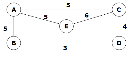
In the weighted graph, the edges are labelled with weights. If the above graph represented the distances between locations, you can quickly calculate the relative cost of different routes between the locations. The weights can be negative numbers - remember the graph is an abstract representation of a real-world scenario.

There is interest in determining the shortest path between vertices - you should look for Dijkstra's algorithm online and be thankful you haven't been asked to pronounce the name out loud.

Directed Graphs

A directed graph includes arrows on each edge. The arrows show the path that can be followed from each vertex to the next. Be careful of getting bogged down in the map model though. The arrows can be used to represent other facts.

In the diagram below, the vertices represent teams playing a round-robin tournament. Each team plays each of the others once.

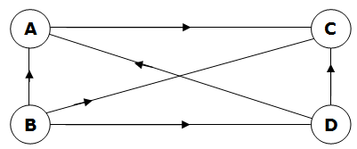
The arrow on each edge shows which of the two connected teams won the match. In this diagram, team A beat team C but lost to team B. Team B won the tournament since they were the only undefeated team.

Adjacency Matrix - Undirected Graph

An adjacency matrix is a way of representing the connections in a graph.

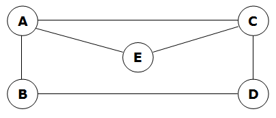
The adjacency matrix for the above graph is as follows,

	A	B	C	D	E
A	0	1	1	0	1
B	1	0	0	1	0
C	1	0	0	1	1
D	0	1	1	0	0
E	1	0	1	0	0

In the table, a 1 is used to indicate that the vertices are connected, a 0 is used where they are not. For a directed graph, the adjacency matrix is symmetrical. For example, there is a 1 for the connection from A to E and for the connection from E to A.

Adjacency Matrix - Directed Graph

Our round-robin tournament graph will not have a symmetrical adjacency matrix. For example, A is adjacent to C but not to B.

	A	B	C	D
A	0	0	1	0
B	1	0	1	1
C	0	0	0	0
D	1	0	1	0

Reading the table row-by-row, we clearly see that team B are the winners of this tournament and that team C didn't win a match.

Adjacency Matrix - Weighted Graph

In a weighted graph, the weights need to be accounted for in the adjacency matrix. Since 0 might be a valid weight, we cannot use that to represent the absence of an edge. Infinity tends to be used in such cases.

	A	B	C	D	E
A	∞	5	5	∞	5
B	5	∞	∞	3	∞
C	5	∞	∞	4	6
D	∞	3	4	∞	∞
E	5	∞	6	∞	∞

Adjacency List - Undirected Graph

An adjacency list details the neighbours of each vertex.

Vertex	Adjacent Vertices
A	B, C, E
B	A, D
C	A, D, E
D	B, C
E	A, C

Adjacency List - Directed Graph

With a directed graph, the adjacency list must take into account the direction of the arrows on each edge.

Vertex	Adjacent Vertices
A	C
B	A, B, D
C
D	A, C

Adjacency List - Weighted Graph

The adjacency list for the weighted graph must include details of the weight of each edge.

Vertex	Adjacent Vertices
A	B,5; C,5; E,5
B	A,5; D,3
C	A,5; D,4; E,6
D	B,3; C,4
E	A,5; C,6

Graph Traversal - Depth-First Search

A path is a sequence of vertices beginning at one vertex, visiting a series of vertices until the destination is reached. A depth-first search of a graph begins with one vertex and follows a path from there until it reaches the last vertex. It then backtracks and follows a different path from the initial vertex. It does this until all vertices are reached.

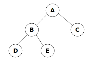
When we perform this kind of search, we need to keep track of whether or not we have visited a vertex (discovered) and whether or not we have fully explored a vertex. A depth-first traversal of the above graph would run as follows,

Step 1 - Start With Vertex A

Vertex	Discovered	Completely Explored
A	True	False
B	False	False
C	False	False
D	False	False
E	False	False

Stack (Bottom To Top): A

Step 2 - Visit A's First Neighbour

Vertex	Discovered	Completely Explored
A	True	False
B	True	False
C	False	False
D	False	False
E	False	False

Stack (Bottom To Top): A, B

Step 3 - Visit B's First Neighbour

Vertex	Discovered	Completely Explored
A	True	False
B	True	False
C	False	False
D	True	True
E	False	False

Stack (Bottom To Top): A, B, D

Step 4 - Backtrack And Visit B's Second Neighbour

Vertex	Discovered	Completely Explored
A	True	False
B	True	True
C	False	False
D	True	True
E	True	True

Stack (Bottom To Top): A, B, E

Step 5 - Backtrack And Visit A's Second Neighbour

Vertex	Discovered	Completely Explored
A	True	True
B	True	True
C	True	True
D	True	True
E	True	True

Stack (Bottom To Top): A, C

When the discovered and completely explored columns are true for each vertex, the entire graph has been traversed.