Computer Science
Data Representation
Program Design
Hardware & Software
Networks
Databases
Data Structures
Algorithms
Other
![]()


Computer Science
Turing Machines
Turing machines are abstract computational devices first proposed by Alan Turing in 1937. A Turing machine is a theoretical device that manipulates symbols on a strip of imaginary tape. It is an abstract representation of a computing machine that was originally used to explore the limitations and capabilities of computing machines in general.
A Turing machine is an automaton consisting of,
A Tape - the tape is divided into sections or cells, each one capable of storing a symbol. The tape has a left end but can be extended infinitely to the right. Cells without symbols written on them are blank and will contain the blank cell symbol,  . The tape can have symbols read from it and written to it.
A Read-Write Head - the head can read symbols from and write them to the tape. The head can move the tape one cell to the left or right at a time. In diagrams, the head is often more likely to move than the tape -- the effect is the same.
A (Finite) Table Of Instructions - the instructions are the transition function for this machine. Given the current state of the machine, and the symbol currently under the read-write head, the table must show what the machine must do from the following list,
- Write a symbol or erase (write a blank) a symbol on the tape
- Move the head one place to the left or right, or stay in the current position
- Assume the new state - this can be the same state as before
A Set Of Possible States - this set would include the current state of the machine, other states that the machine can assume and must include a set of halting states (accepting states).
Example Of A Turing Machine
The following example is based on the first Turing machine that Alan Turing proposed. The machine has the task of writing 1 0 1 0 1 0... on the tape. The 1s and 0s alternate with an empty cell in between them. We can describe that using the following state transition diagram. Note, there is no halting state in this example - it will carry on writing in this pattern forever,
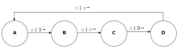
There are 4 states for the machine. State A is the starting point. In State A, the machine reads from the tape, it should read an empty cell. It writes a 1 in that cell, moves one cell to the right and assumes state B. In State B, a blank cell is read from the tape, a blank cell is written back to the tape, the tape moves one to the right and assumes state C. And so on,
The table of instructions for this Turing Machine is as follows,
| Curent State | Scanned Symbol | Print Action | Move Action | Next State |
|---|---|---|---|---|
| A | Blank | 1 | Right | B |
| B | Blank | | Right | C |
| C | Blank | 0 | Right | D |
| D | Blank | | Right | A |
We could write the transition rules for this machine as follows,
δ(A, ) = (B, 1, →)

δ(B, ) = (C, , →)

δ(C, ) = (D, 0, →)

δ(D, ) = (A, , →)
The delta symbol represents the transition function. It is followed by the current state and input symbol. To the right of the equals sign is the next state, symbol to write and direction in which to move the tape.
What's The Point?
This conceptual model of a computing machine is as basic as they get. You cannot divide these operations any futher. This means that any computing machine can be reduced to an equivalent Turing machine. The Turing machine, therefore, can describe the operation of any computing machine. It does this independently of any hardware.
Turing machines are particularly useful for exploring what is and is not computable.
The Busy Beaver Function
The busy beaver function is defined as the largest number of 1s that can be written to a tape by a Turing machine with n states that halts at some point.
There is no algorithm that can calculate whether or not a given Turing machine will halt (see next section for proof).
If you make a one-state Turing machine - one state leading to a stop state which is not counted as part of the busy beaver function, you get exactly one 1 on the tape. This outcome is described symbolically as B(1) = 1. The busy beaver number for a 1-state machine is 1. A two-state Turing machine is described in the diagram below,
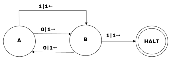
Assuming that our tape is padded out with 0s or blank symbols, 'executing' this machine would have the following effect,
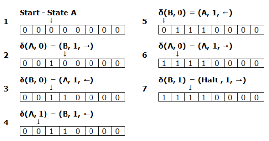
A two-state busy beaver machine can write four 1s onto the tape, B(2) = 4.
A four-state busy beaver leaves 13 marks on the tape. A five state busy beaver produces at least 4098 marks. B(6) is at least 1.29 x 10 865. The numbers become too large to work with from this point onwards.
Universal Turing Machine
When Alan Turing first proposed the idea of the Universal Turing Machine (UTM), it was quite a revelation. The idea is that you have a machine which we will call U. On its tape, it has has the transition rules for another machine which we will call M. It also has on the tape the input data for machine M. Turing's assertion was that machine U would then be able to compute the exact same sequence as M. Machine U simulates the behaviour of other Turing machines when given their transition rules and the input data.
U will probably not execute as quickly as M. By 1966, it was discovered that U would only need be slower than M by a logarithmic factor.
This is similar to the way that an interpreter works on a modern computer. When you point your browser at a PHP web page, a program on the server interprets the instructions in the script, producing the output specified in the program. The web page you see is the result of this interpretation of the instructions written in the script.
The UTM concept is quite powerful when you stop taking for granted the advances in technology that have occurred since that time. One implication is that programs and data are really the same thing - the tape in a UTM contains both the program and the data as a series of symbols. This links very strongly with the stored program concept that we looked at in Comp 2. We see this principle of universality at work with the computers that we use. New applications can be written to enable all sorts of different tasks to be performed by the same machine.